Fractional Brownian motion

This post aims to provide context for, and a brief, accessible overview of, my masters research on fractional Brownian motion. It is structured by the contributions of a series of key figures: Robert Brown, Albert Einstein, Norbert Wiener, Andrey Kolmogorov, Benoit Mandelbrot and (tongue-firmly-in-cheek) me.

Brown

Summer, 1827. The Scottish biologist Robert Brown—who spent the years between 1801 and 1805 circumnavigating Australia with Matthew Flinders—is peering down a microscope, at a sample of pollen particles suspended in pond water.

figure 1 (i) A microscope that belonged to Robert Brown, which is held in the collection of the Linnean Society of London (the photograph is reproduced with their permission). (ii) An attempt by me to observe the same type of motion in pollen grains that Brown initially observed. I used wattle pollen (hence the yellow) on a modern dark-field microscope. Whether this is true Brownian motion is unclear, but it does look something like this. Other more clearly successful attempts, including one using Robert Brown’s own microscope from the photo, are linked in the footnotes^[2].

Having observed the phenomena equally in pollen from all the living plants he had examined, Brown hypothesised that the particles were “male”, and the movement was due to them pruriently seeking “female” pollen with which to reproduce. To test the robustness of his theory, he expanded the scope of his investigation.

If the movement was sexual in nature, then it should not persist for long after the death of the plant. But Brown found that drying or soaking the plants in spirits for a few days had no effect on the motion of their pollen, though by that time they would have been well and truly dead. Dried and preserved plants that had been sitting in a local herbarium for over a hundred years also still exhibited the motion.

Additionally, if the movement was sexual then it should not occur in species that reproduced through other means. Brown tested ground up samples of mosses, in which the existence of sexual organs had not been universally admitted. They still moved.

Needing a new hypothesis, Brown thought that perhaps the motion was a fundamental property of organic tissues. He kept investigating and showed that the movement could be observed in ground up animal tissues, both living and dead.

But this hypothesis also collapsed, as he tested substances with increasingly tenuous connections to living things. The movement was present in substances of loosely “vegetable origin”, such as gum resins, fossilised wood and pit coal. But it was even present in “silicified wood”, so could not be limited to organic bodies.

Over the next few months, Brown tested every substance he could think of: window glass, “many simple earths and metals”, “rocks of all ages”, stalactites, lava, obsidian, pumice, “a fragment of the Sphinx”, volcanic ashes, meteorites, manganese, nickel, plumbago, bismuth, antimony, arsenic, asbestos…

But that was as far as he got. The reasons for the movement remained mysterious.

Einstein

1905 was Einstein’s annus mirabilis, the year in which he published four revolutionary papers on relativity, the equivalence of energy and matter ($e=m{c}^2$), the photoelectric effect and, perhaps least widely known, a proposed explanation for Brownian motion. It went as follows.

Liquid water is effectively a soupy pinball machine of microscopic ${\mathrm{H}}_2\mathrm{O}$ molecules. Each of these molecules is zooming around and bumping into all the others. The temperature of the water is determined by the average speed of the molecules it is made of - the higher the temperature, the faster the molecules are moving, and the more frequently they bump into each other.

When a pollen particle is suspended in water, it too is now being bombarded by all the water molecules that are flying around. Each time a water molecule impacts the pollen grain, it exerts a force on the grain in the direction of impact. If the pollen grain is not too big, and if enough water molecules hit the grain in the same direction at the same time, the grain starts moving in that direction. The sheer number of water molecules enveloping the pollen grain mean that it is constantly being jolted in every direction by the incessant barrage of collisions.

figure 2 This is a simulation of the basic principle^[5]. Hit PLAY to start it running. The small blue dots play the role of water molecules, the large yellow dot is a grain of pollen. Observe how the pollen moves in response to being hit by the water molecules. Use the slider to increase the temperature, which causes the water molecules to move faster. The movement of the pollen becomes more erratic as the frequency of the collisions increases. Finally, click HIDE WATER to make the water molecules invisible. The observed movement of the pollen grain is effectively what can be seen in the microscope footage in Figure 1.

The above simulation is only a simplistic demonstration. In reality, the water molecules would be much smaller relative to the pollen grain, and there would be far more of them. No single collision between a water molecule and the pollen grain would result in observable movement. Instead, each observed jolt is caused “by an enormously large number of successive kicks it receives from different fluid particles which, by rare coincidence, give rise to a net displacement in the same direction”^[6].

Using the kinetic theory of heat (ie. that temperature $\approx$ speed of molecules) as a starting point, Einstein used the postulated sizes of water molecules to predict the size of the movements a particle the size of a pollen grain should, in theory, experience. The predicted size was large enough to be observable under a microscope, but he refrained from making any conclusions about whether his theory was sufficient to explain the motion observed by Robert Brown.

Einstein’s proposed explanation was controversial at the time, because while the existence of atoms had been theorised, it was not universally accepted. Some physicists thought that atoms were merely a useful computational tool, and didn’t correspond to reality. In 1906, one of the chief proponents of atomic theory, Ludwig Boltzmann, felt defeated and committed suicide. But Einstein’s theory provided a means of using the size of observed vibrations to determine the mass and quantity of the “atoms” that had caused them. This experiment was soon carried out by Jean Perrin; the results won him the 1926 Nobel Prize in physics and silenced all remaining skepticism on the existence of atoms.

Wiener

Though Einstein introduced mathematics into the study of Brownian motion, it was only in the context of modelling the physical phenomena of small particles moving erratically in a liquid. Norbert Wiener—a former child prodigy who in the 1940s was already corresponding with union leaders to warn about the risk of intelligent machines replacing human workers^[8]—created a mathematical formulation of Brownian motion that was much more abstract, and hence much more widely applicable.

To appreciate Wiener’s contribution, we need to introduce the concept of a stochastic process. (Stochastic is just a fancy word for random.) A stochastic process is a set of random variables, indexed by a parameter which usually denotes ‘time’ or ‘space’. For example, the cumulative number of busses that have arrived at a bus stop across time, the humidity at each point on Earth, and the price of tuna at the Toyosu Fish Market in Tokyo across time can all be thought of as stochastic processes.

The vertical position (or $y$-coordinate) of a constantly-jiggling pollen grain on a microscope slide, viewed as a function of time, is also a stochastic process. Wiener constructed a mathematical stochastic process, now called the Wiener process, which was an idealised model of the movement of a pollen grain. In mathematical contexts, the term Brownian motion (or Bm) is generally assumed to refer to the Wiener process, rather than to the physical motion that inspired it.

figure 3 This generator allows you to simulate from Wiener’s stochastic process. Hit SIMULATE PATH to simulate a path. Think of the generated path as a graph showing the vertical position of a pollen grain on a microscope slide as a function of time. Note that we need to distinguish between a stochastic process and a sample path or trajectory of the process. A simple analogy is the action of tossing a coin. A ‘stochastic process’ is analogous to ‘the laws of probability that govern all possible coin tosses’, whereas a ‘sample path’ of a stochastic process is analogous to ‘the observed outcome (either heads or tails) of a particular coin toss’. Thus, the lines plotted by this generator are each a sample path of the Wiener process, but the Wiener process itself is the probabilistic laws governing the evolution of all such paths.

The Wiener process is an idealisation of physical Brownian motion because it makes some simplifying assumptions. One assumption is that the direction the particle moves in the future is independent of the direction it has drifted in the past. Another assumption is that the paths of the Wiener process are fractal, meaning that you can zoom in as much as you want and the graph will still be infinitely wiggly.

figure 4 This is what we mean when we say the Wiener process is fractal^[9].

This is not the case for the position of a pollen grain in water because, while there is a truly enormous number of collisions driving the motion, the number is still finite, so there will be some (incredibly tiny) interval of time between each collision during which the pollen drifts in a straight line, unimpeded. Nonetheless, it is a sufficiently close approximation to reality that the model is still useful. And useful for modelling many phenomena beyond the mere jiggling of pollen grains.

Remarkably, Wiener formulated the Wiener process before the modern framework of probability theory was developed. That is, before there were widely accepted definitions for terms like ‘random variable’, ‘expected value’ or ‘probability’, or ‘stochastic process’.

Kolmogorov

Kolmogorov is the guy who made probability respectable.

He also, amongst his prolific output, described (in 1940) a generalisation of the Wiener process that he called the ‘Wiener spiral’, but is today known as fractional Brownian motion (fBm), which was the subject of my thesis. For whatever reason, the generalisation received only limited attention until it was popularised by Mandelbrot 29 years later, so I will explain exactly what fBm is in the following section.

Mandelbrot

Benoit Mandelbrot is perhaps best known for his work on fractals, such as the iconic Mandelbrot set.

figure 5 The Mandelbrot set^[12].

While he didn’t discover fBm, he did coin its modern name (ie. ‘fractional Brownian motion’) and was largely responsible for its popularisation, which stemmed from a paper he co-authored in 1968.

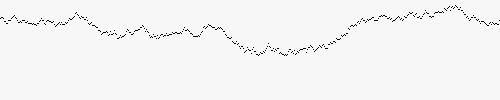
Fractional Brownian motion is a generalisation of the Wiener process, or standard Brownian motion. Technically, fBm is not a single process, but a family of related stochastic processes, one for each number between 0 and 1. This number, called the Hurst parameter and usually denoted $H$, determines the nature of the process. When $H=0.5$, the fBm is simply standard Bm. (This is why fBm is a generalisation of Bm, because it reduces to Bm for a particular value of $H$.) When $H$ is less than 0.5, the sample paths of the fBm are rougher than for Bm. This is because the past is now negatively correlated with the future; if the process has been heading in one direction, it is more likely than not to change direction, and this holds at every point in time. Conversely, when $H$ is greater than 0.5, the sample paths of fBm are smoother than for Bm. This is because the past is now positively correlated with the future; if the process has been heading in one direction, it is more likely than not to keep heading in that direction.

figure 6 This generator allows you to simulate from fractional Brownian motions. Hit SIMULATE PATH to simulate a path. The slide that controls the Hurst parameter is set to 0.5 by default, so the plotted path should look similar (in roughness) to those generated in the standard Brownian motion generator in Figure 3. Now try changing the Hurst parameter using the slider, and generating new sample paths for different Hurst parameters. The sample paths will become increasingly rough as the Hurst parameter approaches zero, and increasingly smooth as the Hurst parameter approaches one.

The advantage of fBm over Bm is that it loses some of the assumptions that do not realistically apply to many of the real-world processes that people are interested in modelling. In particular, the assumption that how the process has evolved in the past doesn’t affect how it evolves in the future does not apply to many real world processes, where there can be underlying trends that persist for long periods of time. This property loosely corresponds to the mathematical concept of ‘long memory’ or ‘long range dependence’, which fBm is capable of modelling for certain values of the Hurst parameter.

Since Mandelbrot’s paper, fBm (and other stochastic processes that are derived from fBm) have been widely used to model time series or spatial data that exhibit fractal properties. Example fields of application include:

• bioengineering - to model regional blood flow distributions in the heart, lungs and kidneys
• communication theory - to model the arrivals of packets of data on a computer network
• hydrology - to model water levels in rivers and the permeability of soils to water
• finance - to model the prices of stocks and other financial instruments
• genetics - to model stochastic gene expression and DNA walks
• Bayesian machine learning - to induce a prior distribution on the space of regression curves
• computer graphics - to generate natural-looking clouds, terrain and cellular noise
• soft matter physics - to model diffusion in crowded fluids
• fluid dynamics - to model the degree to which each point on a turbulent wave front is ‘out of sync’

Thorburn

And so we arrive at my thesis.

For the record, my name is indubitably the odd-one-out in this line-up. Many other probabilists have made significant contributions in the decades since Mandelbrot’s work, which I don’t have time to go into.

Compared to Bm, fBm has a set of features that make it a more realistic process with which to model many phenomena, but those same features also tend to make it harder to work with mathematically. For example, the fact that fBm can have ‘long-range dependence’ means that when calculating probabilties of certain events in the future, you need to account for the influence of how the process has evolved in the past. This is in contrast to standard Bm, where the future is independent of the past, and so the past does not need to be factored into the calculations.

For these reasons, it is important for mathematicians to have access to a diverse pool of representations for fBm, so that when trying to do computations with fBm, they have multiple avenues of approach they can try. Here, I am using the word ‘representation’ in a very specific sense. Namely, a representation of a stochastic process is a formula that takes in one process (in our case, standard Bm), and spits out another process (in our case, fBm).

figure 7 Schematic of a fBm representation formula.

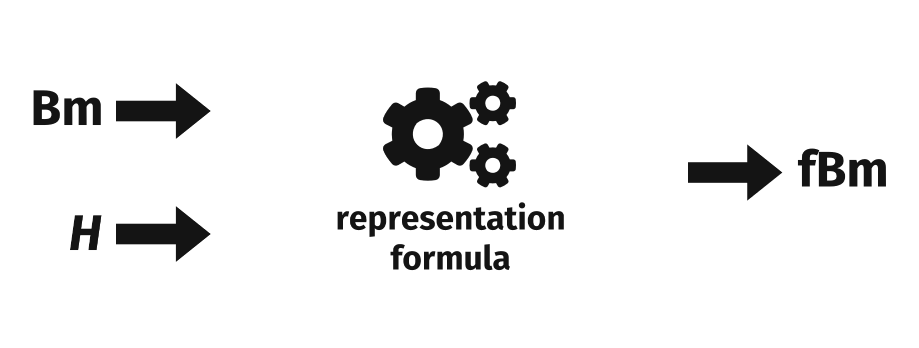
Representations thus provide a link between the world of standard Bm, which probabilists are very familiar with and for which there already exists a comprehensive literature, and the world of fBm, which is more complicated and for which there exists fewer known results. When trying to get a result for fBm, it may be possible to use a representation to convert that result from fBm-world back to standard Bm-world, and prove or derive it there in the more familiar setting, where your toolbox is larger.

My thesis investigated aspects of two representation formulae for fBm: the Muravlev representation, and the Molchan-Golosov representation. The properties of the Muravlev representation I investigated are fairly technical, so I point you to my thesis if you would like to know more. But I can say a bit more about my work on the Molchan-Golosov representation.

With a particular abstract definition of a helix, we can show that fractional Brownian motion is a helix. (This is why Kolmogorov originally called it the Wiener spiral.) This helix exists in an infinite-dimensional space, so it is impossible to visualise it perfectly. Nonetheless, to get the basic intuition, picture a helix in the shape of a simple metal spring. Fractional Brownian motion is that helix. When the Hurst parameter $H$ is such that the fBm is rough, and more likely than not to turn back on itself at every point in time, the helix is more tightly coiled. When the Hurst parameter is such that the fBm is smooth, and more likely than not to continue in the same direction at every point in time, the helix is less tightly coiled.

My research suggests that the Molchan-Golosov representation, which turns standard Bm into fBm, has a geometric interpretation. Specifically, it takes the helix corresponding to standard Bm, and either constricts or relaxes it until it reaches the curvature required to be the requested fBm. I was able to prove that this intuition holds in a discrete-time setting, and showed with computer simulation that it appeared to also hold for the Mochan-Golosov representation, which works in a continuous-time setting.

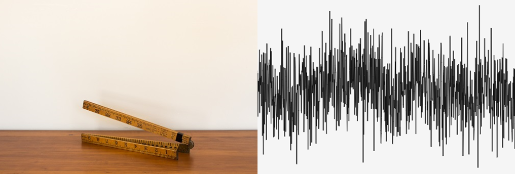
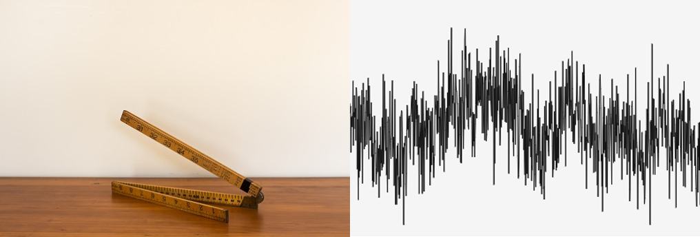
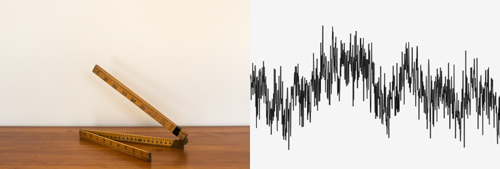
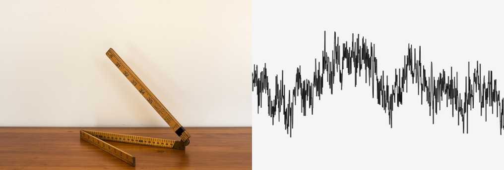
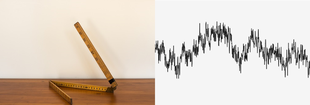
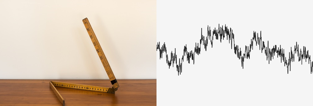
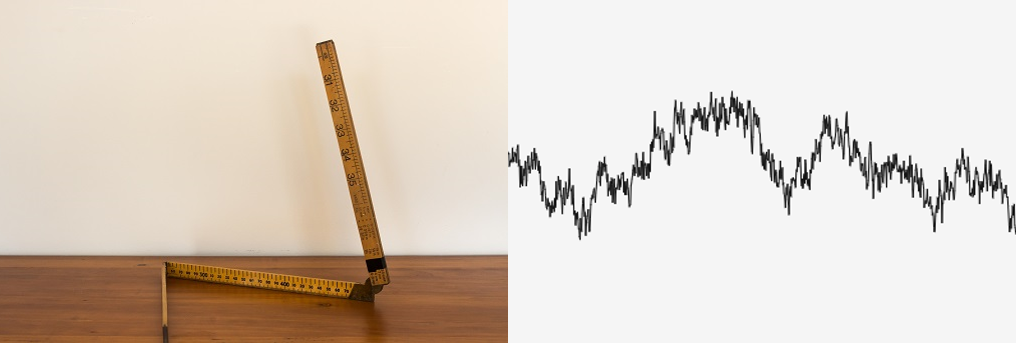
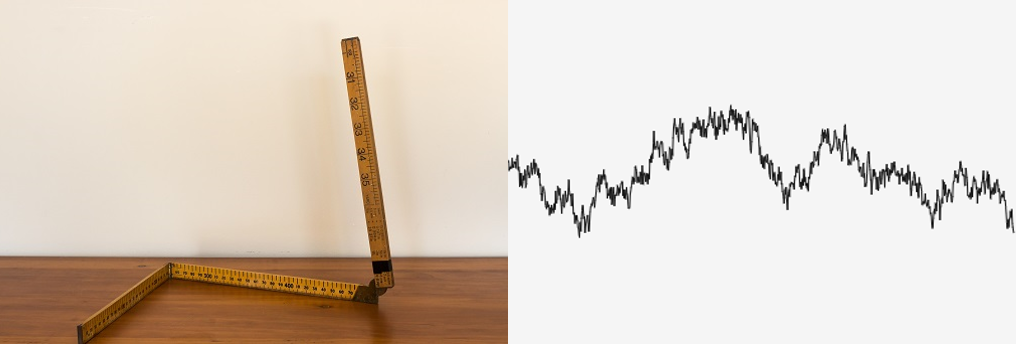
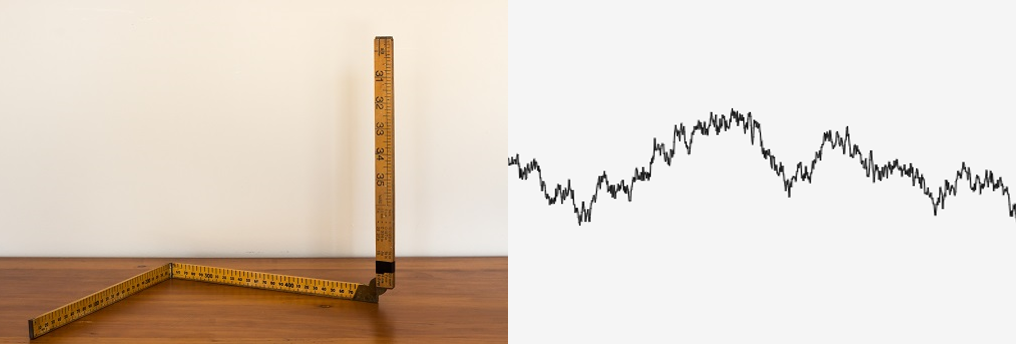
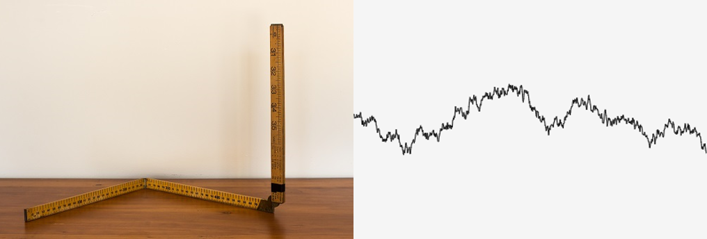
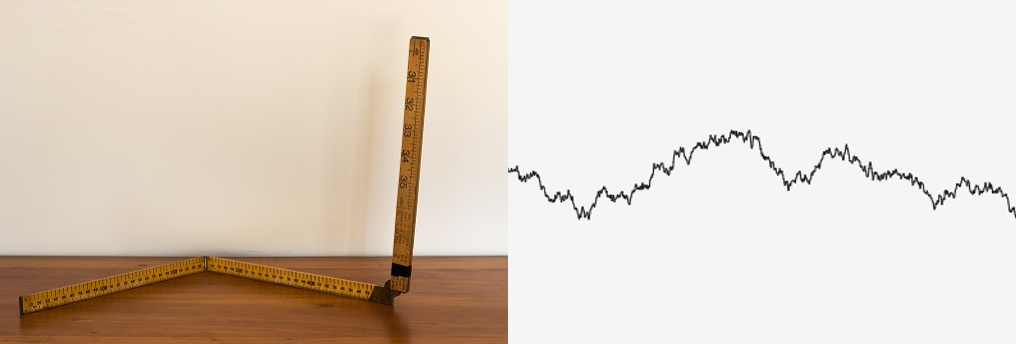
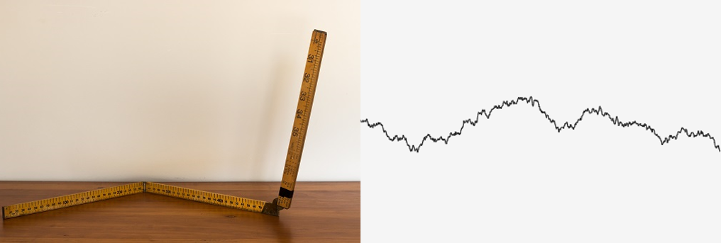
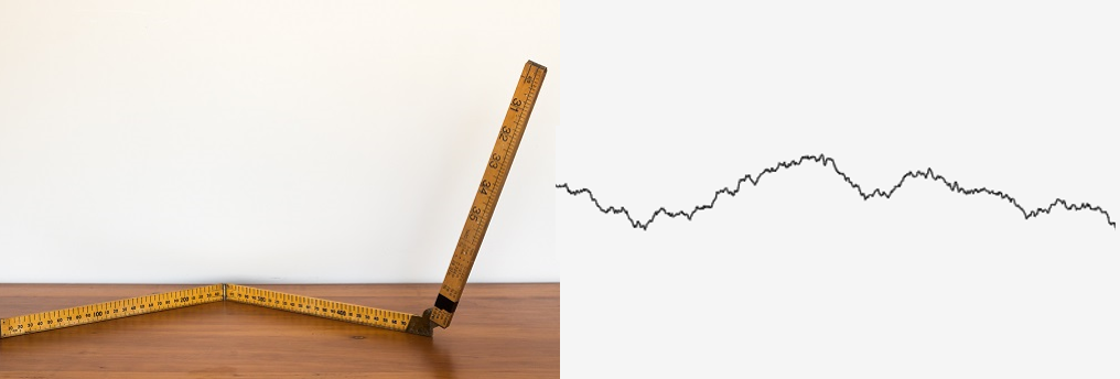
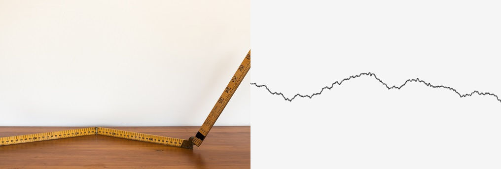
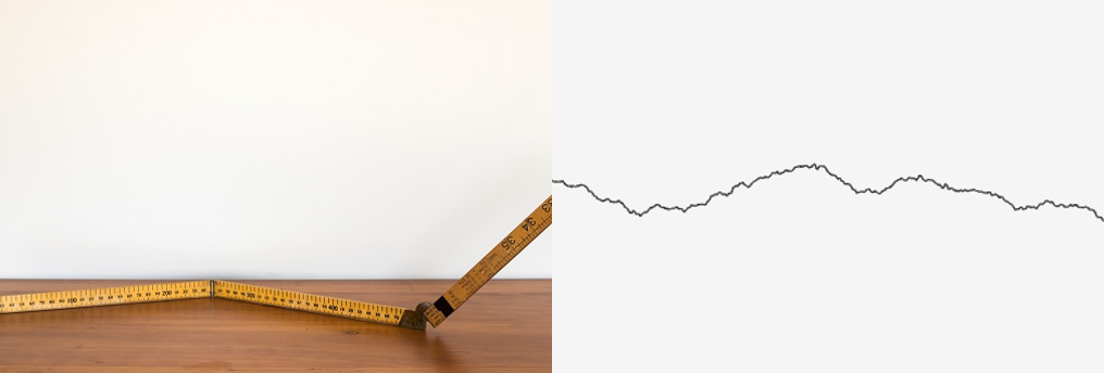
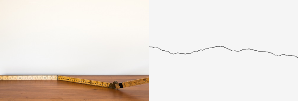
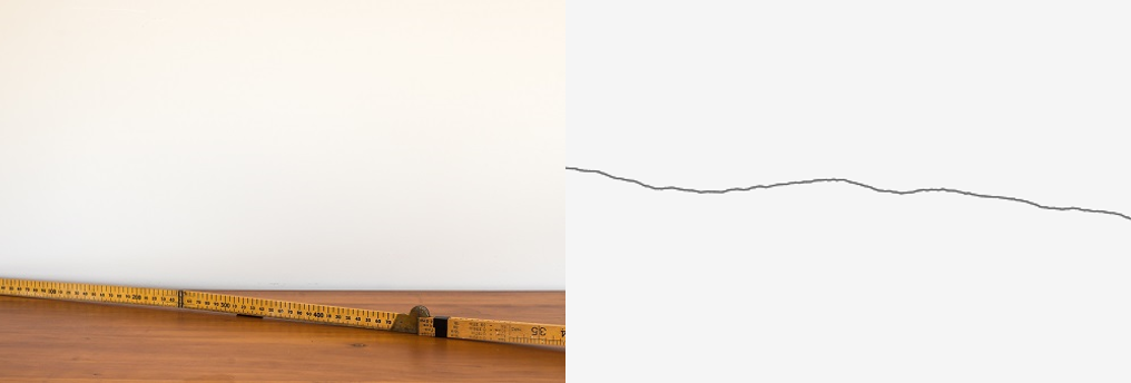
figure 8 Slide the Hurst parameter slider back and forth to get the general intuition. The left panel shows three sections of a discretised helix (I can only show three because we can only visualise three-dimensional space.) The panel on the right shows a simulated fBm sample path. At smaller Hurst parameters, when the path is rougher, the helix coils back on itself. But as the Hurst parameter increases, the path becomes more smooth and the helix relaxes into a straight line.

In sum, my contribution to the theory on fractional Brownian motion was to

• further understanding of some technical properties of the Muravlev representation, and
• propose some plausible geometric intuition for the action of the Molchan-Golosov representation.